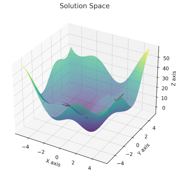
Gradient Descent is a foundational algorithm in machine learning that is essential for training various models, mainly neural networks. It is an optimization strategy, guiding models to minimize error or loss. At its core, Gradient Descent operates on the principle of iterative improvement. The algorithm starts with initial estimates for the parameters of a model and then incrementally adjusts them to find the combination that minimizes the error. It uses the gradient, a mathematical concept representing the direction and rate of the fastest increase of a function, to navigate the multi-dimensional landscape of the model’s error function.
The Gradient Descent Process
- Error Function and Its Importance: The error function, or the cost or loss function, quantifies how far a model’s predictions are from the actual outcomes. In the context of Gradient Descent, it’s the terrain we navigate to find the lowest point, representing the smallest error. While the appropriate error function may be relatively easy in simple models like linear regression, how do you best quantify the error in image classification if the model classifies an image of pizza as a cat? It’s wrong, but how bad? Is it better to classify pizza as bread?
- The Gradient and How It’s Computed: The gradient is the vector of partial derivatives of the error function for each parameter. Computing it involves calculating how much a slight change in each parameter affects the error. This calculation is pivotal, as it points each parameter’s vector in the direction where the function decreases most steeply.
- The Descent: Step Size and Direction: Gradient Descent moves in the opposite direction of the gradient, towards lower error. The step size, controlled by the learning rate parameter, determines each step’s size. If the steps are too large, the algorithm might overshoot the minimum; if too small, the process becomes slow and may get stuck in local minima. The art of Gradient Descent lies in balancing these factors to efficiently reach the lowest point of the error function.
Introduction to Error and Loss Functions
Error and loss functions are fundamental to machine learning, acting as the guiding stars for models during their training phase. These functions quantify the difference between the predicted outputs of a model and the actual target values, offering a measurable way to evaluate and improve model performance.
Types of Loss Functions Used in Machine Learning
Different machine learning problems call for other loss functions. Here are some commonly used ones:
- Mean Squared Error (MSE): A staple in regression tasks, MSE measures the average squared difference between the estimated and actual values. It’s handy when larger errors are more significant, as the squaring operation emphasizes larger differences (in addition to making all values positive).
- Cross-Entropy: Widely used in classification tasks, cross-entropy measures the difference between two probability distributions - the actual distribution and the model predictions. It’s especially effective in scenarios where the prediction of the probability of a class is required.
- Hinge Loss: Often used in support vector machines (SVMs, a ML method) and some types of neural networks, particularly for “maximum-margin” classification. Huber Loss: A combination of MSE and Mean Absolute Error, it’s less sensitive to outliers than MSE.
- Logistic Loss: Used in logistic regression, measuring the difference between binary or multiclass labels and predictions.
Optimizers and Advanced Gradient Descent Techniques
Optimization algorithms vary in their approach to navigating the loss landscape. Remember, not only do we not know what the entire landscape looks like (all the algorithms know is from where I stand now, how can I move to a lower point), but it is highly dimensional. Navigating the hyperdimensional universe in the dark can be a challenge! Here’s a look at some common types:
- Stochastic Gradient Descent (SGD): This algorithm represents the simplest form of gradient descent. It updates the model’s weights using only one sample at each iteration. While this can make SGD faster and more memory-efficient, it can also make the optimization path noisy and inconsistent.
- Batch Gradient Descent: This algorithm simultaneously updates the model parameters using the entire dataset. Unlike SGD, which updates parameters using only one data point at a time, batch gradient descent computes the average gradient from all data points, leading to more stable and consistent parameter updates. However, this can be computationally intensive for large datasets and less efficient than SGD.
- Mini-batch Gradient Descent: Striking a balance between batch gradient descent and SGD, this approach uses a subset of the data at each step. This middle ground makes it more stable than SGD and often more efficient than using the entire dataset.
Momentum-based Optimizers:
- Adam (Adaptive Moment Estimation): Adam combines the ideas of momentum (considering past gradients) and adaptive learning rates (adjusting the learning rate for each parameter) to make more effective updates.
- RMSprop (Root Mean Square Propagation): This optimizer dynamically adjusts each parameter’s learning rate, making it effective for problems with noisy or sparse gradients.
Advanced Concepts:
- Learning Rate Decay: Over time, reducing the learning rate can help the optimizer settle into the minimum of the loss function. This technique is especially useful to prevent overshooting in the later stages of training.
- Adaptive Learning Rates: Algorithms like Adam and RMSprop adjust the learning rate for each parameter, which can lead to more effective training by customizing the step size based on the behavior of each parameter.
Choosing the Right Optimizer: A Guide
Selecting the right optimizer for a specific problem can significantly impact model performance. Here are some guidelines:
- Consider optimizers like Adam or RMSprop for sparse data, as they handle noise well.
- Traditional SGD can be effective and easier to control for simpler models or smaller datasets.
- Experiment with different learning rates and observe the training process. Sometimes, a combination of optimizers used in different training phases can yield the best results.
- Stay informed about the latest developments in optimization algorithms, as this is an actively evolving area in machine learning research.


