- Forward Pass: Input data is passed through the network layer by layer, using the current weights and biases to produce a prediction. In the last module, we had a model that could predict the class of a picture fed to it. During the training process, the forward pass was feeding images into the model and letting it guess what it “thought” it was “seeing.”
- Loss Calculation: The network’s prediction is compared to the actual target values using a loss function, quantifying how far off the predictions are. In the pizza recognizer example, if the model guessed that a picture of a pizza was a “cat,” the loss function would tell the model it needed to adjust its weights and biases and try again.
- Backward Pass (Backpropagation): The gradient of the loss function concerning each weight and bias is computed. We aren’t going to dive into the details, but this uses partial differential equations (from that Calculus class you may have taken long ago) to find the gradients (or tangents). These gradients indicate the direction and magnitude to adjust each parameter (weights and biases) to minimize the loss calculated by the loss function.
- Optimization: Weights and biases are adjusted to decrease the loss. The learning rate, a hyperparameter, determines the size of the adjustments. This step is the secret sauce for how networks learn: With each backward pass, the network (hopefully) gets a little more accurate with its predictions.
- Iterative Process: The forward pass, loss calculation, backpropagation, and optimization steps are repeated multiple times (epochs) on the training data until the network converges to an optimal set of weights and biases or until a set number of epochs is reached.

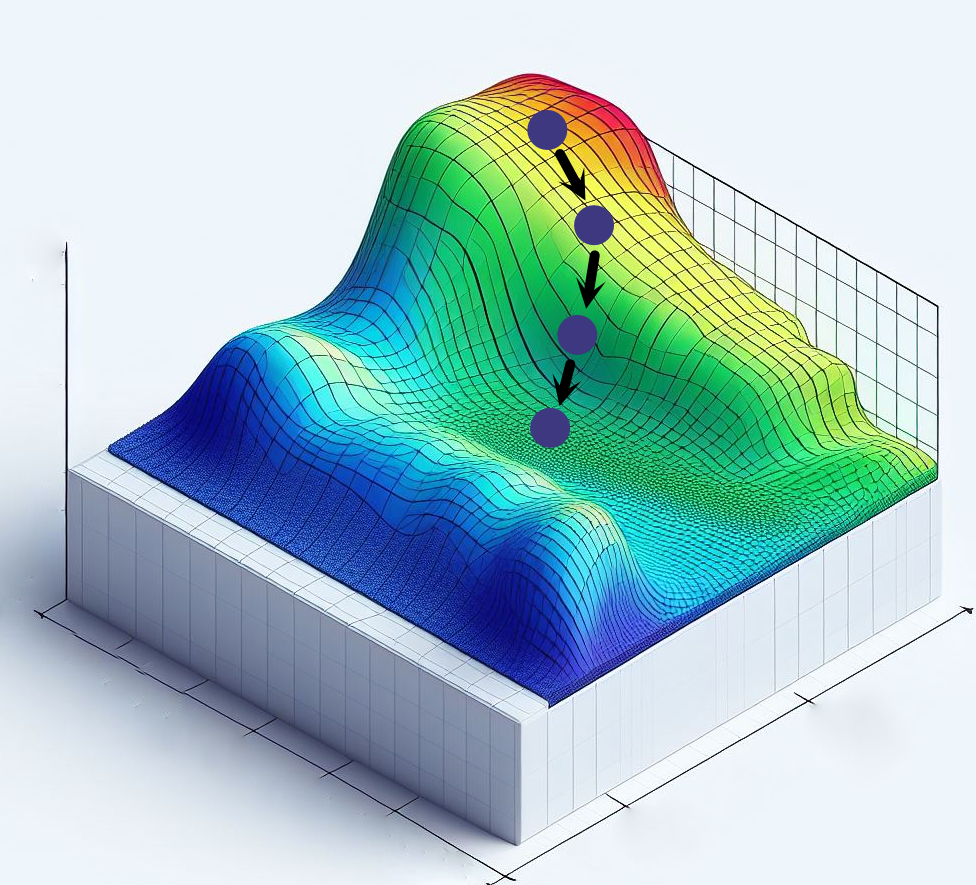
The 3D surface in this figure represents the loss surface for different sets of weights. While we draw this in 3D, this surface is highly dimensional, with as many dimensions as there are parameters (millions!). At each epoch, the loss is calculated. Each blue dot is the position on the loss surface at an epoch. The gradient and learning rate are used to calculate the direction and amount each parameter should be adjusted. The training data are re-evaluated, and the new loss is calculated. This process iterates repeatedly until the loss reaches a satisfactory level.


