Accuracy is a starting point, but it often hides the true story. Computer vision tasks come with unique challenges: rare objects, critical decisions where a single false positive is disastrous, or dealing with datasets where some classes dominate others. Choosing the right metrics is key to improvement.
- Class Imbalance: If you’re detecting a rare type of defect on an assembly line, knowing that your model is 95% accurate means little if it misses most of those defects! Precision and recall will expose this issue (see definitions below).
- Object Detection Trade-Offs: Are you building a security system? Perhaps catching every potential threat is paramount, even at the cost of some false alarms. You’d focus primarily on recall.
Visualize What Your Model ‘Sees’
Tools like confusion matrices, saliency maps, and Grad-CAM let you peer into your model’s decision-making process. These are crucial for debugging and building trust:
- Confusion Matrix: This matrix reveals where your model excels and stumbles. Does it consistently mistake one type of object for another? That’s your cue to target that problem with specialized data collection or tailored augmentations.
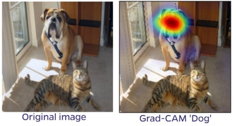
- Saliency Maps: Saliency maps show you what parts of the image your model considers most important. Is it confusing a cat for a dog because both have ears? Or has it learned the correct features? This exposes potential biases or unintended shortcuts your model might have picked up.
- Grad-CAM: (Gradient-weighted Class Activation Mapping) is a technique used to visualize which regions of an image are important for a neural network’s prediction. Similar to Saliency Maps, it works by using the gradients of the target class flowing into the final convolutional layer to produce a heatmap. This heatmap highlights the areas of the image that the model focused on when making its decision, helping interpret the model’s behavior.
Evaluation Metrics for Different Tasks
Here we’ll cover which evaluation metrics are the most common for each major computer vision task. You’ll hopefully recognize many of these from the last notebook!
Classification
- Accuracy: A good starting point but can be misleading in imbalanced datasets.
- Precision & Recall: Essential for imbalanced classes. Precision tells you how many of your predicted positives are correct (avoiding false positives). Recall tells you how many of the actual positives your model captured (avoiding false negatives).
- F1-Score: A balanced metric combining precision and recall into a single score.
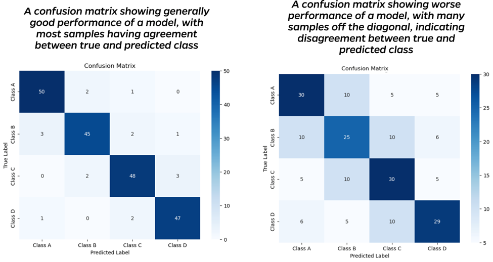
- Confusion Matrix: A matrix showing how often your model confuses classes. The confusion matrix on the left below shows that most inputs are correctly categorized. Ideally, all values would be on the diagonal, indicating agreement between the true and predicted labels. The image on the right shows a worse-performing model, with many off-diagonal values.
-
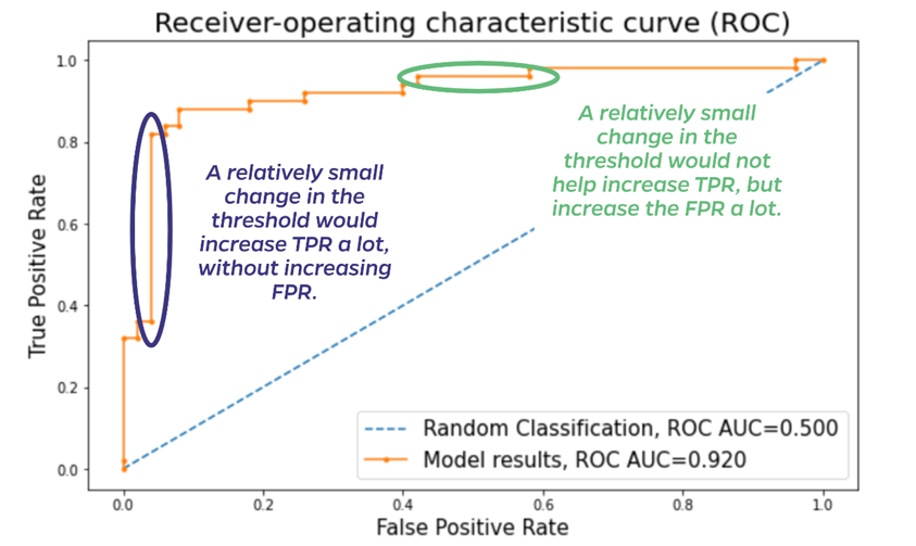
ROC-AUC Curve: Useful when dealing with class imbalance. It shows the trade-off between true positive rate (correctly identified positives) and false positive rate (incorrectly identified positives) at various thresholds. A higher AUC-ROC score indicates better performance.
The image below illustrates a typical receiver-operating characteristic (ROC) curve. The diagonal line indicates random classification and has an area under the curve (AUC) of 0.5. The AUC will increase as the curve moves up and to the left, indicating a generally better model. The points along the curve plot the true positive rate (TPR) and false positive rate (FPR) for different classification thresholds. If classifying cats and dogs, for example, and a model predicts a probability of 0.7 for a sample being a dog, one threshold would be 0.5 (anything over 0.5 probability is a dog). But one could also set the threshold to be 0.8—only classify as dogs samples predicted with 0.8 or higher probability. You might want to be more sure it’s a dog before assuming it will use the litter box for example! Where to set the threshold depends on the consequences of incorrect predictions. The ROC helps evaluate the impact of changing the threshold. While the thresholds themselves are not shown on the plot below, each dot is a different threshold, and the threshold decreases from left to right. In addition to the overall AUC of 0.92, the ROC curve highlights areas like those circled in blue and green. The blue oval highlights a place where decreasing the threshold dramatically increases the TPR (a good thing), while leaving the FPR relatively unchanged. If applying this model, one would certainly want to use the lower threshold. Conversely, the green oval highlights a region where decreasing the threshold only increases the FPR (a bad thing) without any increase in TPR. That change in threshold would have only negative consequences in using the model.
Object Detection
- Mean Average Precision (mAP): A common metric that considers both precision and recall across different object categories and Intersection over Union (IoU) thresholds (how well your bounding box overlaps the actual object).
- Average Precision (AP): Similar to mAP but for a single object category.
- Precision-Recall Curves: Similar to ROC-AUC curves but visualize the trade-off between precision and recall for object detection tasks.
- Visualization Tools: Bounding box visualizations help identify issues like missed objects, inaccurate bounding boxes, or over-detection.
Segmentation
- Pixel-Level Accuracy: Measures the percentage of pixels correctly classified in your segmentation masks.
- IoU: Similar to object detection but measures the overlap between predicted and ground truth segmentation masks.
- Mean Intersection over Union (mIoU): The average IoU across all classes in your segmentation task.
- Visualization Tools: Visualize predicted segmentation masks alongside ground truth masks to identify regions where the model struggles or makes consistent errors. Tools like class activation maps (CAMs) can highlight which image features the model relies on for segmentation tasks.
Tips for Smarter Iteration
- Understandable Baseline: Before deploying a complex solution, start small. It might surprise you, and even if it performs poorly, it’ll often clearly reveal shortcomings to solve before moving to fancier techniques.
- Think About Your Problem: What really matters for your task – speed, precision on a specific class, overall accuracy? Tailor your evaluation accordingly. Organized Experimentation: Keep detailed records of your experiments. Track the metrics with tools like TensorBoard, of course, but also store those results. They’ll prove invaluable when comparing models or trying to understand why a past change improved results.
Return to Module 3 or Continue to Troubleshooting Common Computer Vision Problems
